
One may run into a situation that calls for numerical differentiation of some quantity along a curve in a 2D parameter space. That is, we have a curve parameterized by 1D variable t that draws out a path in a 2D (x,y) space; and we want the derivative f'(x,y)\equiv f'(t) of the quantity f(x,y) along the curve. In this post, I demonstrate a way to do this using finite differences.
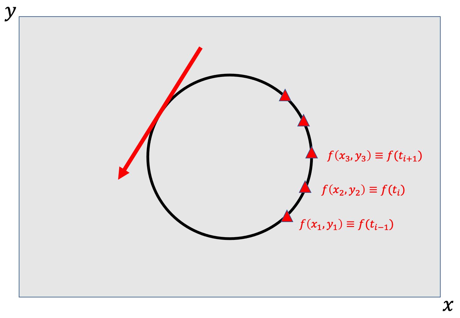
Strictly writing, f(x,y) is a 1D array of data objects (e.g., numbers, matrices) that are given in some order. This means that the parameter t needn’t necessarily represent time; it can be any quantity that introduces some notion of ordering to preserve the sequential nature of the data along the path (so that we know which point comes next). For example: f(x,y) = \{f(x_1,y_1), f(x_2,y_2), f(x_3,y_3), … f(x_N,y_N)\}\equiv \{f(t_1), f(t_2), f(t_3), … f(t_N)\} , where (x_i, y_i) and t_i are fixed values, as in the figure below. Note that the difference \Delta t_i between each t_i needn’t be constant.

Practical cases that yield f(x,y) :
- An experimentalist gives you a set of data for some quantity they measured along a 2D curve. Example: f(x,y) \equiv Berry phase as a magnetic field is used to move an electron in a curve. Or, the body temperature of an ant as it frantically revolves in a circle around a dead bug.
- A program calculates some complicated quantity at (x,y) coordinates that draw out a curve, into an array. Example: f(x,y) \equiv a 2D time-independent Hamiltonian H(x,y) matrix. So, each data ‘point’ in f(x,y) \equiv can be a matrix, if you want to calculate the derivative of the matrix along the loop (for computing other quantities such as \Bra{\psi} \frac{dH(t)}{dt}\Ket{\psi} .
- You have an annoying algebraic equation f(x,y) whose derivative you cannot calculate analytically to get a closed form (or it’s not worth the effort trying to get). So, you just find its value at (x,y) coordinates that draw out a curve. For whatever reason, you could still do this with a simple equation like f(x,y) = x^2 + 2 y^3. But, you might as well just take the derivative analytically and plug in the (x,y) coordinates to get your derivative f'(x,y) .
For specificity, let’s start with case 3 above, since it has the most steps of the three. The other two cases will follow the same logic once f(x,y) is acquired.
Let’s begin by considering a circular curve (closed loop). We are interested in the derivative of our quantity f(x,y) as it traces the path along the curve parameterized by t . A circle of radius r , centered at (x_0,y_0), can have the 1D parameterization: \{x(t) = x_0+r\cos(t), y(t) = y_0+r\sin(t)\}. Then, we can get the 1D representation: f(x,y) \equiv f(x(t),y(t)) \equiv f(t) . That is, if we use the example equation f(x,y) = x^2 + 2 y^3, we get f(t) = (x_0+r\cos(t))^2 + 2(y_0+r\sin(t))^3.
For a complete circle, t\in[0,2\pi]. So, we can calculate the values of f(t) along the loop by evaluating it at points along the loop. For instance, we can discretize the loop into segments. For convenience, I break the loop into equal-sized segments. For instance, if I choose \Delta t = 0.1, I will have \{f(0), f(0.1), f(0.3), … f(2\pi)\}. f(x,y) is now acquired. Needless to say, if you have the freedom to choose this interval, a smaller \Delta t will give you a higher resolution, but potentially at the cost of more computational resources.
Now, regardless of which of the 3 cases you are dealing with, you can proceed to get an approximate derivative using finite differences for numerical differentiation. There’s a lot of accessible literature online on the theory behind this. I extract the following from Alice C. Yew’s lecture notes. There are three popular kinds of finite differences for first-order derivatives: forward differences, backward differences and central differences. I use the latter because it makes me feel emotionally safe. Oh and, because, when considering the three methods’ simplest forms, the latter’s error is second-order O(\Delta z^2) instead of being first-order O(\Delta z) like the other two. That is, it is better. However, please note that there are different, lengthier equations that give better errors for forward and backward differences.
The idea is that you calculate the following quantity for each point on your curve. In our case, the standard equations translate to:
f'(t)=\frac{f(t_{i+1}) - f(t_{i-1})} {2\Delta t}
A programming implementation then becomes clear: You iterate through each point on your loop to calculate this. The previous figure illustrates these choices of t_i .
Let’s use Python to do this for our simple example! Hopefully the comments help explain what’s going on. One could easily rewrite this code into a different programming language: The logic is the same.
Start by importing libraries:
import numpy as np
import matplotlib.pyplot as plt
Got data already? That is, cases 1 and 2:
my_data = np.random.rand(100) # Generate dummy data set for example.
n_segs = my_data.shape[0]-1 # Number of line segments is 1 less than the number of points

### Calculate derivative f'(x,y) numerically ###
df_loop = np.zeros(n_segs) # Create empty array for values of f'(x,y)
for i in np.arange(1,n_segs): # Notice we start from index 1 and not the Python's first index 0, because the first point does not have a f(t_{i-1}) 'previous' value!
    f2 = my_data[i+1] # Value at 'next' (x,y) point
    f0 = my_data[i-1] # Value at 'previous' (x,y) point
    df = (f2-f0)*(n_segs/(4*np.pi)); # n_segs/(4*np.pi) = 2\Delta t in the provided equation. Please change this as necessary if all step intervals are not constant, or somehow different. This could be an array of different values itself.
    df_loop[i-1] = df
No existing data? That is, case 3:
### Define constants ###
n_pts = 100 # Number of points to discretize to. The number of line segments is then (n_pts-1).
x0 = 0; y0 = 0; # Coordinates of circle center (x0,y0)
r = 0.5; # Radius of circle

### Parameterize 2D space curve ###
# Define t values. E.g., (0, 0.1, 0.2, ..., 2\pi), depending on n_segs:
t = np.linspace(0, 2*np.pi, num=n_pts) # t goes from 0 to 2\pi for a complete circle.
# Append the second t point to the end, so that the central difference can be calculated at the last point. Because, the sequentially 'next' value f(t_{i+1}) is required:
t = np.append(t,t[1])
# Create empty array for coordinates of 2D space loop (x,y) and assign its values using 1D parameterization of circle. Notice that we have (n_pts+1) entries as we added an extra point above.
k_loop=np.zeros((n_pts+1,2))
for i in range(n_pts+1):
    k_loop[i,:]=np.array([x0 + r*np.cos(t[i]), y0 + r*np.sin(t[i])])

### Define function ###
def my_f(loop): # "loop" is an array of coordinates (x1,y1)
    x=loop[0]; y=loop[1];
    return x**2 + 2*y**3 #

### Calculate derivative f'(x,y) numerically ###
df_loop = np.zeros(n_pts) # Create empty array for values of f'(x,y)
for i in np.arange(1,n_pts): # Notice we start from index 1 and not the Python's first index 0, because the first point does not have a f(t_{i-1}) 'previous' value!
    f2 = my_f(k_loop[i+1]) # Value of my_f at 'next' (x,y) point
    f0 = my_f(k_loop[i-1]) # Value of my_f at 'previous' (x,y) point
    df = (f2-f0)*(n_pts/(4*np.pi)); # n_pts/(4*np.pi) = 2\Delta t in the provided equation. Please change this as necessary if all step intervals are not constant, or somehow different. This could be an array of different values itself
    df_loop[i-1] = df
Visualize either case:
fig = plt.figure()
ax = plt.axes()
ax.plot(df_loop)
plt.xlabel("t",fontsize=20);
plt.ylabel("f '(x,y)",fontsize=20);
plt.show()
For the case 3 example, you’ll get something like this. Nice, smooth derivative.

Goodbye.