
The time-independent Schrödinger equation appears in several applications of quantum mechanics. In this post, I will go over how I numerically calculate energy dispersions of such matrix equations. What this boils down to is solving for the eigenvalues of a matrix equation, the time-independent Schrödinger equation:
H |n\rangle = E_n |n\rangle
For an N-level system, H above is an N\times N matrix specified by the system under consideration. |n\rangle are instantaneous eigenstates of the system (i.e. eigenvectors to those familiar with linear algebra), and E_n are the energy eigenvalues we desire to find.
In this post, I will focus on contexts often seen in condensed matter physics: two-dimensional tight-binding models written in terms of momentum-space k=(k_x,k_y) variables. This makes H,|n\rangle and E_n functions of k. Our underlying k-space domain is then a first Brillouin zone with periodic boundary conditions.
For illustration, let us focus on the simple model for graphene with an on-site potential. This model describes the well-renowned gapless graphene, but allows for an on-site potential M to gap the system. While I leave details of this model to these notes, I will simply use the Hamiltonian they provide:
H(k,M)=-t \sum\limits_{\delta} [\cos(k\cdot\delta)\sigma_x-\sin(k\cdot\delta)\sigma_y+M\sigma_z]
Plugging in the Pauli matrices \sigma_x,\sigma_y,\sigma_z, the above is nothing but:
H(k,M)=-t \sum\limits_{\delta} \begin{pmatrix} M & \cos(k\cdot\delta)+i \sin(k\cdot\delta) \\ \cos(k\cdot\delta)-i \sin(k\cdot\delta) & -M \end{pmatrix},
where \delta_1=\frac{a}{2}(1,\sqrt{3}), \delta_2=\frac{a}{2}(1,-\sqrt{3}), and \delta_3=-a(1,0) . For completeness, I mention that \delta_i are nearest-neighbor lattice vectors, a the lattice constant, and t the nearest-neighbor hopping parameter.
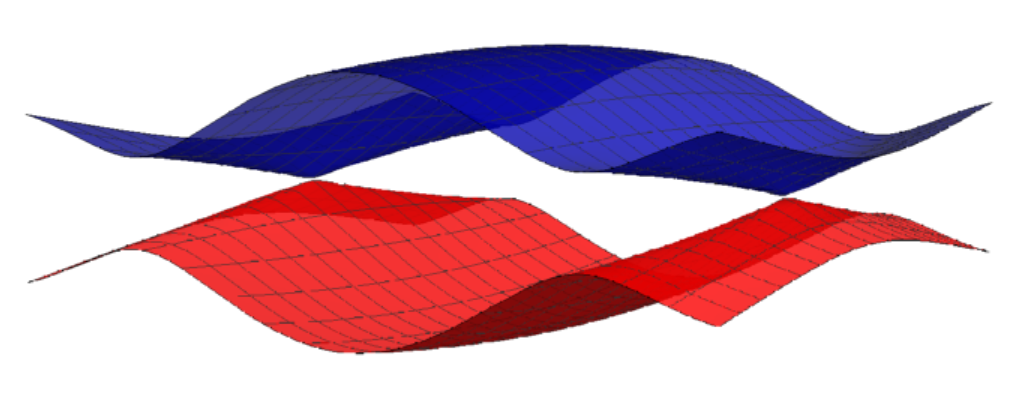
This 2\times 2 Hamiltonian is a 2-level Hamiltonian that yields 2 instantaneous eigenvectors/wavefunctions corresponding to 2 eigenvalues. In the figure below, the eigenvalues pertaining to each eigenvector are shown in two different colors (red and blue). As a sanity check, notice the two gapless Dirac points expected for graphene’s dispersion (i.e. where the eigenvalues touch / are degenerate)!

To generate energy band diagrams like the one above, you simply have to solve for the Hamiltonian’s eigenvalues at each k-point in k-space. You may find these eigenvalues ‘analytically’ (to find expressions for the eigenvalues using algebra, that you can then plug k-points into), or ‘numerically’ (evaluating the Hamiltonian at each k-point first, to numerical get eigenvalues directly). Analytical solutions are often restricted to simple systems, making numerical solutions more favorable.
With all this machinery in hand, I now present commented code for both approaches: Mathematica for the analytical approach, and Python and MATLAB for the numerical one. Note that the MATLAB and Python routines are the same, and that the Mathematica code provides the most comments on parameter choices. To test other Hamiltonian systems, simply replace the definitions of the Hamiltonians below!
Challenge: Try changing the following code to play with the Haldane model for the quantum anomalous Hall effect! One possible momentum-space Hamiltonian is given by equations 34 (with equation 4) in this review: An Introduction to Topological Insulators.
Mathematica
(* choose k-space region (usually 1st Brillouin zone): *)
BZx1 = -0.3; BZx2 = 0.3; BZy1 = -1.3; BZy2 = 1.3;
(* on-site mass, lattice constant and hopping: *)
M = 0; a = 2.46; t = 1; (* M=0 is for graphene *)
(* nearest-neighbor vectors: *)
delta1 = a/2 {1, Sqrt[3]}; delta2 =
 a/2 {1, -Sqrt[3]}; delta3 = -a {1, 0};
(* k: *)
k = {kx, ky};
(* Pauli matrices: *)
sx = {{0, 1}, {1, 0}}; sy = {{0, -I}, {I, 0}}; sz = {{1, 0}, {0, -1}};
(* Hamiltonian: *)
hx = Cos[k.delta1] + Cos[k.delta2] + Cos[k.delta3];
hy = Sin[k.delta1] + Sin[k.delta2] + Sin[k.delta3];
hz = M;
H[kx_, ky_] = -t (hx*sx - hy*sy + hz*sz);
(* analytic expressions for energies: *)
eigenvals[kx_, ky_] = Eigenvalues[H[kx, ky]];
(* plot *)
Show[Plot3D[
  eigenvals[kx, ky][[1]], {kx, BZx1, BZx2}, {ky, BZy1, BZy2},
  PlotStyle -> {Red, Opacity[0.8]}],
 Plot3D[eigenvals[kx, ky][[2]], {kx, BZx1, BZx2}, {ky, BZy1, BZy2},
  PlotStyle -> {Blue, Opacity[0.78]}]]
Python
This implementation requires the Python packages NumPy and Matplotlib.
import numpy as np
from numpy import linalg as LA
import matplotlib.pyplot as plt

# First, define your Hamiltonian.
# The following function returns the Hamiltonian matrix for input (kx,ky).
def Hamiltonian_Graphene(kx,ky,M):
    a = 2.46
    t = 1
    k = np.array((kx,ky))
    delta1 = (a/2)*np.array((1,np.sqrt(3)))
    delta2 = (a/2)*np.array((1,-np.sqrt(3)))
    delta3 = -a*np.array((1,0))
    sx = np.matrix([[0,1],[1,0]]);
    sy = np.matrix([[0,-1j],[1j,0]]);
    sz = np.matrix([[1,0],[0,-1]]);
    hx = np.cos(k@delta1)+np.cos(k@delta2)+np.cos(k@delta3)
    hy = np.sin(k@delta1)+np.sin(k@delta2)+np.sin(k@delta3)
    hz = M
    H = -t*(hx*sx - hy*sy + hz*sz)
    return H

# Onto plotting the dispersion.
# The parameters m,n specify the resolution to discretize the parameter space into (e.g. break it into m=100 pieces in the kx direction).
# The parameters BZx1,BZx2,BZy1,BZy2 specify the edges of your parameter space.
def plot_dispersion(M,m,n,BZx1,BZx2,BZy1,BZy2):
    # Generate a mesh
    kx_range = np.linspace(BZx1, BZx2, num=m)
    ky_range = np.linspace(BZy1, BZy2, num=n)
    # Get the number of levels with a dummy call (an NxN square matrix has N levels)
    num_levels = len(Hamiltonian_Graphene(1,1,1))
    energies = np.zeros((m,n,num_levels)); # initialize
    # Now iterate over discretized mesh, to consider each coordinate.
    for i in range(m):
        for j in range(n):
            H = Hamiltonian_Graphene(kx_range[i],ky_range[j],M);
            evals, evecs = LA.eig(H); # Numerically get eigenvalues and eigenvectors
            energies[i,j,:]=evals;
    X, Y = np.meshgrid(kx_range, ky_range) # Generate actual mesh for plotting.
    # Plot! There are several ways to style this.
    fig = plt.figure()
    ax = fig.gca(projection='3d')
    ax.axis([X.min(), X.max(), Y.min(), Y.max()])
    transparency = 0.3 #transparency
    for band in range(num_levels):
        ax.scatter3D(X, Y, energies[:,:,band], alpha=transparency, antialiased=False, label="c")
    plt.show()

# Run it!
M=0
BZx1 = -0.3; BZx2 = 0.3; BZy1 = -1.3; BZy2 = 1.3;
plot_dispersion(M,100,100,BZx1,BZx2,BZy1,BZy2)
MATLAB
Define the following 3 functions in separate .m files, then run the code in the last block using the Command Window (or a script).
% Hamiltonian:
function [H] = Hamiltonian_Graphene(kx,ky,M)
    a = 2.46; t = 1;
    k = [kx,ky];
    delta1 = (a/2)*[1, sqrt(3)];
    delta2 = (a/2)*[1, -sqrt(3)];
    delta3 = -a*[1, 0];
    sx = [0,1;1,0];
    sy = [0,-1i;1i,0];
    sz = [1,0;0,-1];

    hx = cos(k*delta1')+cos(k*delta2')+cos(k*delta3');
    hy = sin(k*delta1')+sin(k*delta2')+sin(k*delta3');
    hz = M;
    H = -t*(hx*sx - hy*sy + hz*sz);
end
% function to generate k-space grid:
function mesh = meshsq(m,n,BZx1,BZx2,BZy1,BZy2,offsetx,offsety)
kx = linspace(BZx1,BZx2,m+1);
ky = linspace(BZy1,BZy2,n+1);
mesh = zeros(m,n,4,2);
for i = 1:1:m
for j = 1:1:n
mesh(i,j,1,:) = [kx(i),ky(j)];
mesh(i,j,2,:) = [kx(i+1),ky(j)];
mesh(i,j,3,:) = [kx(i+1),ky(j+1)];
mesh(i,j,4,:) = [kx(i),ky(j+1)];
end
end
end% function to get energies at each k-space point:
function [e1,e2] = PlotDispersion_2Band(BZx1,BZx2,BZy1,BZy2,m,n,M)
% get grid of k-points to calculate energies for
mes = meshsq(m,n,BZx1,BZx2,BZy1,BZy2);
% initialize energies
e1 = zeros(m,n);
e2 = zeros(m,n);
for i=1:1:m
for j = 1:1:n
H = Hamiltonian_Graphene(mes(i,j,1,1),mes(i,j,1,2),M);
eigs = eig(H);
e1(j,i) = eigs(1,:);
e2(j,i) = eigs(2,:);
end
end
end% Run the following using the Command Window (or a script) to plot!
M=0;
BZx1 = -0.3; BZx2 = 0.3; BZy1 = -1.3; BZy2 = 1.3;
m_mesh = 100; n_mesh = 100;
[e1,e2] = PlotDispersion_2Band(BZx1,BZx2,BZy1,BZy2,m_mesh,n_mesh,M);
figure; hold on
surf(e1, 'FaceColor','b', 'FaceAlpha',0.7, 'EdgeColor','none')
surf(e2, 'FaceColor','r', 'FaceAlpha',0.7, 'EdgeColor','none')
hold offDisclaimer: I reserve the right to oppose every accusatory point you make in action against me.