
There are several techniques one could use to extract exchange interactions J using DFT calculations (e.g., 4-state energy mapping). In this tutorial, we will extract isotropic exchange J for NN, 2NN and 3NN interactions by fitting spin-spiral energies from VASP to a spin-1/2 Heisenberg model on a triangular lattice.
Spin-spiral calculations are a powerful approach to model long-wavelength magnetic excitations using only a primitive unit cell, rather than large supercells. They rely on imposing a spatially modulated magnetic structure characterized by a propagation vector q, such that the magnetic moment at position \mathbf{r} + \mathbf{R} is given by:
\mathbf{m}(\mathbf{r} + \mathbf{R}) = \begin{pmatrix} m_x(\mathbf{r}) \cos(\mathbf{q} \cdot \mathbf{R}) - m_y(\mathbf{r}) \sin(\mathbf{q} \cdot \mathbf{R}) \\ m_x(\mathbf{r}) \sin(\mathbf{q} \cdot \mathbf{R}) + m_y(\mathbf{r}) \cos(\mathbf{q} \cdot \mathbf{R}) \\ m_z(\mathbf{r}) \end{pmatrix}
By computing the total energy for different q vectors, one can fit the dispersion to a Heisenberg spin model and extract isotropic exchange parameters J for various neighbor distances (e.g., NN, 2NN, 3NN). This method is especially advantageous because it avoids the need for multiple magnetic configurations and large supercells required by approaches like the 4-state energy mapping method.
However, a notable limitation of spin-spiral calculations in VASP is that they currently cannot include spin–orbit coupling (SOC) due to the use of the generalized Bloch theorem (gBT). As a result, only collinear and non-relativistic interactions can be studied directly in this framework.
Methodology Overview
- Calculate the spin-spiral energies for q vectors along a high-symmetry path (e.g., \Gamma\rightarrow K \rightarrow M \rightarrow \Gamma \rightarrow M_1 \rightarrow M_2 ; where M_i are different M points (which are usually symmetry-equivalent unless symmetry is broken via strain, for instance; coordinates in Python code below). I used VASP for this step.
- Numerically fit these energies to the spin-1/2 Heisenberg model. In this tutorial we work with a 2D triangular lattice, up to 3NN interactions (i.e., we get J_1, J_2, J_3). I used Python for this step.
You may choose your own workflow to do the above. With the intention of potentially positively influencing your workflow, I am sharing mine below. I had to do several of these fittings to investigate my research problem, and so I carried out calculations in bulk. Below, I am assuming familiarity with VASP.
Step 1: DFT
- First, in the parent directory, create a file qpoints with the coordinates of the q vectors. For the path \Gamma\rightarrow K \rightarrow M \rightarrow \Gamma \rightarrow M_1 \rightarrow M_2 , you could use the following Python code to generate a list of 86 q vectors (which I interchangeably call ‘q points’ since each is a list of 3D coordinates):
import numpy as np
# Define k-point path G M K G M1 M2 with appropriate intervals between segments
segments = [
    (np.array([0, 0, 0]), np.array([0.5, 0, 0]), 20), # G to M1
    (np.array([0.5, 0, 0]), np.array([0.333333, 0.333333, 0]), 15), # M to K
    (np.array([0.333333, 0.333333, 0]), np.array([0, 0, 0]), 25), # K to G
    (np.array([0, 0, 0]), np.array([0.5, 0.5, 0]), 15), # G to M1
    (np.array([0.5, 0.5, 0]), np.array([0, 0.5, 0]), 15), # M2 to M2
]
# Generate k-points and write to qpoints file
with open("qpoints", "w") as f:
    last_point = None
    for start, end, num_points in segments:
        for point in np.linspace(start, end, num_points):
            rounded_point = tuple(round(coord, 6) for coord in point)
            if rounded_point != last_point:
                f.write(f"{rounded_point[0]} {rounded_point[1]} {rounded_point[2]}\n")
                last_point = rounded_point
- Configure the VASP input files for your spin-spiral calculation in a folder called template (which should contain INCAR, KPOINTS, POSCAR, POTCAR and a Slurm script for job submission which I call sc). These files are the same as an scf calculation’s but with the additional tags for spin-spirals. We will next use a script to make a copy of this template folder for each separate q point and run each calculation. The template directory should be in the same directory level as the qpoints file. Carefully read the VASP documentation here. Some notes:
- You need to set:
- LNONCOLLINEAR = .TRUE.
- LSPIRAL=.TRUE.
- ENINI = … (see documentation for guidance)
- ENMAX = … (see documentation for guidance)
- MAGMOM = … (e.g., 1 0 0 1 0 0 1 0 0 24*0 for Nb3I8 with magnetic Nb atoms and non-magnetic I atoms; see this tutorial for more on setting MAGMOM in noncollinear cases). In this tutorial, we set magnetic ions with MAGMOM in the x-direction (i.e., 1 0 0). This affects the fitting function we use in Step 2.
- In theory, you should set QSPIRAL as well (see documentation for guidance). But in my workflow, I will use a script to later add this tag when running the calculation for each q vector. You are welcome to use a different workflow to specify q.
- You cannot use spin-orbit coupling, as mentioned previously.
- If the spin-spiral curves you get at the end don’t look right (e.g., discontinuous), play around with EDIFF, ENCUT, ENINI, ENMAX. I found my curves to be sensitive to these parameters.
- You need to set:
- Once the template files are set, use the following bash script to make a copy of template for each q point in qpoints, set the corresponding QPSIRAL tag in INCAR, change the name of the Slurm job (for tracking the job), submit the job and move onto the next q point. Reminder: copy-paste this to a new file (e.g., run.sh), change permissions using chmod +x run.sh, and then ./run.sh.
#!/bin/bash
# Loop over k-points from qpoints file
q=1
while read -r kx ky kz; do
    # Create new folder
    cp -r template "$q"
    # Modify files in the new folder
    cd "$q"
    # Add job name to "sc" file
    sed -i "1a #SBATCH --job-name=s0-$q" sc
    # Add QSPIRAL to "INCAR"
    echo "QSPIRAL= $kx $ky $kz" >> INCAR
    # Submit job
    sbatch sc
    # Return to the parent directory
    cd ..
    # Increment folder name
    ((q++))
done < qpoints- Wait for the jobs to finish running. If your cluster has a checkpoint queue, I would recommend using it if the job will finish within the time limit. The current workflow performs 86 calculations for the 86 q vectors.
- It is a good idea to make sure all calculations finished successfully. Since there are many calculations, I would check a few random ones to make sure the calculation has finished as expected. I also use the following script to print the last line of each OUTCAR file in a single file directory_last_lines.txt; in the VASP version I use (6.4.1), a completed calculation ends with a line that looks like “Voluntary context switches: 37738” (the number at the end will differ for different calculations). Just do something to make sure the calculation’s completed as expected and that you can rely on the extracted energy.
#!/bin/bash
# Output file to store the results
output_file="directory_last_lines.txt"
# Clear the output file if it exists
> "$output_file"
# Loop through directories named 1 to 86
for dir in {1..92}; do
    if [ -f "$dir/OUTCAR" ]; then
        # Get the last line of the OUTCAR file
        last_line=$(tail -n 1 "$dir/OUTCAR")
        # Append the directory number and last line to the output file
        echo "$dir: $last_line" >> "$output_file"
    else
        # If OUTCAR does not exist, note it in the output file
        echo "$dir: OUTCAR file not found" >> "$output_file"
    fi
done
echo "Results written to $output_file"- Finally, we can extract the list of energies per q point to a file quick_output.csv for use in the fitting. I use this script (which extracts energy(sigma->0) values; change this script appropriately to extract other energies like energy without entropy if they are more relevant to your case):
#!/bin/bash
# Output file
output_file="quick_output.csv"
> "$output_file"  # Clear the output file if it exists
# Loop through directories 1 to 86 corresponding to each q point
for main_dir in {1..86}; do
    # Check if the required file exists
    if [[ -f "$main_dir/OUTCAR" ]]; then
        # Extract energy(sigma->0)
        energy_sigma=$(grep -a -e "energy(sigma->0)" "$main_dir/OUTCAR" | tail -n 1 | awk '{print $NF}')
        # Write directory number and energy to output file
        echo "$energy_sigma" >> "$output_file"
    else
        # Handle missing files
        echo "$main_dir MISSING_FILES" >> "$output_file"
    fi
done
echo "Output written to $output_file"
Step 2: Numerical Fitting
- Now that we have the spin-spiral energies, we have to numerically fit them to the isotropic spin-1/2 Heisenberg model. Below, \mathbf{S}_i are the spin-1/2 operators, which in this case are proportional to \mathbf{m}(\mathbf{r} + \mathbf{R}) above. The sums are taken over two sites i and j, with the superscripts 1, 2, 3 indicating 1st nearest-neighbor (NN), 2NN and 3NN interactions. Although we truncate the sum to 3NN, you can include an arbitrary number of NN interactions. J_i are the isotropic exchange interaction constants.
H = \frac{1}{2} \left( J_1 \sum_{i,j}^{(1)} \mathbf{S}_i \cdot \mathbf{S}_j + J_2 \sum_{i,j}^{(2)} \mathbf{S}_i \cdot \mathbf{S}_j + J_3 \sum_{i,j}^{(3)} \mathbf{S}_i \cdot \mathbf{S}_j \right)
- If we set magnetic ions to be in the x-direction, then (m_x(\mathbf{r}),m_y(\mathbf{r}),m_z(\mathbf{r}))=(1,0,0), and with \mathbf{S}_i=S^2(m_x(\mathbf{r}),m_y(\mathbf{r}),m_z(\mathbf{r})) for the magnitude of the spin operator (S=1/2 in this case):
\mathbf{S}_i =S \mathbf{m}(\mathbf{r} + \mathbf{R_i}) = S ( \cos(\mathbf{q} \cdot \mathbf{R_i}), \sin(\mathbf{q} \cdot \mathbf{R_i}), 0 )
- Then, for site i at a reference point \mathbf{R_i}=(0,0,0)=\mathbf{0} and site j at \mathbf{R_j}:
\mathbf{S}_i \cdot \mathbf{S}_j = S^2\cos(\mathbf{q}\cdot(\mathbf{0}-\mathbf{R_j}))=\cos(\mathbf{q}\cdot\mathbf{R_j})
- This means that we can fit our spin-spiral energies E to the function:
E=\frac{1}{2} S^2 \left( J_1 \sum_{j}^{(1)} \cos(\mathbf{q}\cdot\mathbf{R_j}) + J_2 \sum_{j}^{(2)} \cos(\mathbf{q}\cdot\mathbf{R_j}) + J_3 \sum_{j}^{(3)} \cos(\mathbf{q}\cdot\mathbf{R_j}) \right)
- In this example, we consider a 2D triangular lattice, which has 6 of each vectors \mathbf{R_j} (with j=1,2,3) corresponding to NN, 2NN and 3NN interactions respectively (see figure below):

- Then, making sure to treat q in terms of reciprocal lattice vectors \mathbf{b_i}, \mathbf{q} = q_x \mathbf{b_1} + q_y \mathbf{b_2} (note: we ignore the z-coordinate since we are dealing with 2D), we can use the following Python code to fit the spin-spiral energies to extract {J_i} and plot the data and fitted function.
import pandas as pd
import numpy as np
from scipy.optimize import least_squares
import matplotlib.pyplot as plt
# Load the Excel file with columns qx, qy (from qpoints file), and E (corresponding spin-spiral energies)
file_path = "data.xlsx" # Change this appropriately
sheet_name = "spin-spirals" # Change this appropriately
data = pd.read_excel(file_path, sheet_name=sheet_name)
# Extract columns
qx = data['qx'].values
qy = data['qy'].values
E = data['E'].values
data = pd.read_excel(file_path, sheet_name=sheet_name)
# Lattice constant and lattice vectors for triangular lattice
a = 6.744 # Change this to reflect your crystal structure
a1 = a * np.array([1, 0])
a2 = a * np.array([-0.5, np.sqrt(3)/2])
b1 = np.array([6.283185307179587, 3.627598728468436])/a # from VASP OUTCAR, or just calculate reciprocal vectors using a1 and a2 above yourself
b2 = np.array([0., 7.255197456936872])/a
# Convert q-points to physical wavevectors using b1 and b2
q_physical = np.array([qx[i] * b1 + qy[i] * b2 for i in range(len(qx))])
# Define R1, R2, R3 vectors (6 of each for triangular latice)
R1_cartesian = np.array([a1, -a1, a2, -a2, a1 + a2, -(a1 + a2)])
R2_cartesian = np.array([a1 + 2 * a2,2 * a1 + a2,a1 - a2,-a1 - 2 * a2,-2 * a1 - a2,-a1 + a2])
R3_cartesian = np.array([2 * a1, -2 * a1,2 * a2, -2 * a2,2 * (a1 + a2), -2 * (a1 + a2)])
# Spin magnitude
S = 1/2; S2 = S**2
# Heisenberg energy model
def extended_energy(q, J1, J2, J3, E0):
qx, qy = q[:, 0], q[:, 1]
cos_q_d1 = sum(np.cos(qx * R[0] + qy * R[1]) for R in R1_cartesian)
cos_q_d2 = sum(np.cos(qx * R[0] + qy * R[1]) for R in R2_cartesian)
cos_q_d3 = sum(np.cos(qx * R[0] + qy * R[1]) for R in R3_cartesian)
return E0 + 1/2 * S2 * (J1 * cos_q_d1 + J2 * cos_q_d2 + J3 * cos_q_d3)
# Define residuals function
def residuals(params, q, E_data):
J1, J2, J3, E0 = params
E_model = extended_energy(q, J1, J2, J3, E0)
return E_data - E_model
# Initial guess for parameters; choice doesn't really affect results in my systems, but are needed for the fitting function
initial_guess = [0.5, 0.1, 0.05, np.min(E)]
# Perform least squares fitting
result = least_squares(residuals, initial_guess, args=(q_physical, E))
# Extract fitted parameters
J1, J2, J3, E0 = result.x # E0 is constant shift, whose value doesn't affect shape of curve and Ji
print("Fitted Parameters (meV):")
print(f"J1 = {1000*J1:.3f}")
print(f"J2 = {1000*J2:.3f}")
print(f"J3 = {1000*J3:.3f}")
print(f"E0 = {1000*E0:.3f}")
# Calculate fitted energies
E_fitted = extended_energy(q_physical, J1, J2, J3, E0)
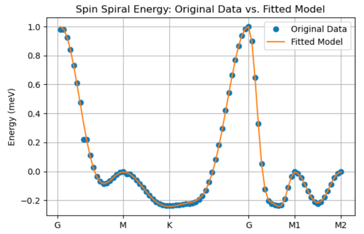
# Plot original vs fitted data
plt.figure(figsize=(6, 4))
plt.plot(range(len(E)), 1000*E, 'o', label='Original Data')
plt.plot(range(len(E_fitted)), 1000*E_fitted, '-', label='Fitted Model')
#plt.xlabel('q-path')
plt.ylabel('Energy (meV)')
plt.title('Spin Spiral Energy: Original Data vs. Fitted Model')
x_ticks = [0, 20, 34, 58, 72, 86] # x values for the labels
x_ticks = [x - 1 for x in x_ticks]
x_labels = ['G', 'M', 'K', 'G', 'M1', 'M2'] # Corresponding labels
plt.xticks(x_ticks, x_labels)
plt.legend()
plt.grid()
plt.tight_layout()
plt.show()- The code above should give a figure like the one below, for which I have J_1 = 0.782, J_2 = 0.224, J_3 = 0.322 meV. In the case below, I got a good fit, indicating the magnetism is accurately described by these exchange interactions.

- Before ending this tutorial, I mention that you can include other terms to the fitting function, such as DMI, which would be incorporated by a term like D \sin(\mathbf{q}\cdot \mathbf{R_j}) in the above example, which can be derived from D\cdot(\mathbf{S_i}\times \mathbf{S_j}). Another aside is that we can use the spin-spiral dispersion to help determine the magnetic ground state of the system, as discussed in this tutorial.
Hope you found this useful!