How to visualize real-space spin texture generated by spin-spirals on a 2D triangular lattice

Spin-spiral dispersions may be used to identify the magnetic ground state of a system. When the spin-spiral energy is plotted as a function of the spin-spiral propagation vector \mathbf{q}, the \mathbf{q} vector corresponding to the energy minimum indicates the magnetic ground state:

\mathbf{q} vector	Ground State
\Gamma=(0,0)	ferromagnetic
K=(1/3,1/3)	120^\circ order
M=(1/2,0)	stripe antiferromagnetic
other	incommensurate

Consider, for instance, the dispersion below, which shows a minimum at the M point, indicating a stripe ground state:

One way to model spin spirals in DFT is to use the generalized Bloch theorem. Click here to see how it is implemented in VASP. From the VASP documentation, the magnetization density behaves as follows, with the components of the magnization in the xy-plane rotating about the spin-spiral propagation vector \mathbf{q}, and \mathbf{R} is a lattice vector:

\mathbf{m}(\mathbf{r} + \mathbf{R}) = \begin{pmatrix} m_x(\mathbf{r}) \cos(\mathbf{q} \cdot \mathbf{R}) - m_y(\mathbf{r}) \sin(\mathbf{q} \cdot \mathbf{R}) \\ m_x(\mathbf{r}) \sin(\mathbf{q} \cdot \mathbf{R}) + m_y(\mathbf{r}) \cos(\mathbf{q} \cdot \mathbf{R}) \\ m_z(\mathbf{r}) \end{pmatrix}

How do we visualize the spin texture in real-space with this information? This is what this tutorial addresses.

Let’s say that we perform our spin-spiral calculations with MAGMOM = 1 0 0 for the magnetic atoms. Then, we have (m_x,m_y,m_z)=(1,0,0). We can then use the equation above to visualize the spin texture in real-space by plugging in \mathbf{q} and \mathbf{R}.

The Python code below shows how this could be accomplished for up to 3 nearest-neighbors in a 2D triangular lattice. If you don’t care about the atom spacing, all you need to do to visualize a spin texture is to change the variable ‘q’ to match your desired ‘q’ point (e.g., where the spin-spiral energy is a minimum).
To elaborate on what’s going on, bear in mind that we need to use \mathbf{q} in terms of the reciprocal lattice vectors \mathbf{b}_1 and \mathbf{b}_2, and not, e.g., q=M=(1/2,0) directly. One could get these reciprocal lattice vectors using known relationships between the primitive lattice vectors \mathbf{a}_1,\mathbf{a}_2 and \mathbf{b}_1,\mathbf{b}_2. But could also easily extract that information numerically from VASP’s OUTCAR file, as done for the code below:

import numpy as np
import matplotlib.pyplot as plt

# Parameters
mx, my, mz = 1, 0, 0

# Define S[q, R]
def S(q, R):
    q_dot_R = np.dot(q, R)
    return np.array([
        mx * np.cos(q_dot_R) - my * np.sin(q_dot_R),
        mx * np.sin(q_dot_R) + my * np.cos(q_dot_R)
    ])

# Lattice Vectors
a = 6.744
a1 = a * np.array([1, 0])
a2 = a * np.array([-0.5, np.sqrt(3) / 2])

# Reciprocal lattice vectors (hardcoded)
b1 = np.array([6.283185307179587, 3.627598728468436]) / a
b2 = np.array([0., 7.255197456936872]) / a

# Nearest Neighbors
R1 = np.array([[0, 0], a1, -a1, a2, -a2, a1 + a2, -(a1 + a2)])
R2 = np.array([a1 + 2 * a2, 2 * a1 + a2, a1 - a2, -a1 - 2 * a2, -2 * a1 - a2, -a1 + a2])
R3 = np.array([2 * a1, -2 * a1, 2 * a2, -2 * a2, 2 * (a1 + a2), -2 * (a1 + a2)])

# Fixed q-point ### !!! CHANGE THIS TO DESIRED q-POINT
q = np.array([0, 0.5])  # Example q-points: [0,0], [0,0.5], [0.5,0], [1/3,1/3], [0.5,0.5]
q_physical = q[0] * b1 + q[1] * b2

# Calculate S[q, R] for each R1, R2, R3
S1 = np.array([S(q_physical, R) for R in R1])
S2 = np.array([S(q_physical, R) for R in R2])
S3 = np.array([S(q_physical, R) for R in R3])

# Scale factor to increase arrow length
scale_factor = 3

# Function to plot arrows
def plot_arrows(R, S, color, label=None):
    plt.scatter(R[:, 0], R[:, 1], color=color, label=label)
    for i in range(len(R)):
        normalized_S = scale_factor * S[i] / np.linalg.norm(S[i]) if np.linalg.norm(S[i]) != 0 else S[i]
        plt.arrow(
            R[i, 0], R[i, 1], normalized_S[0], normalized_S[1],
            color=color, head_width=0.5, head_length=0.7
        )

# Generate individual plots for R1, R2, and R3
plt.figure(figsize=(8, 8))
plot_arrows(R1, S1, 'black', label="R1")
plot_arrows(R2, S2, 'black', label="R2")
plot_arrows(R3, S3, 'black', label="R3")

# Combine all plots
plt.gca().set_aspect('equal', adjustable='box')
plt.xlim(-20, 20)
plt.ylim(-20, 20)
plt.xlabel("X")
plt.ylabel("Y")
plt.title("Real-space Spin Texture")
#plt.legend()
plt.grid(False)
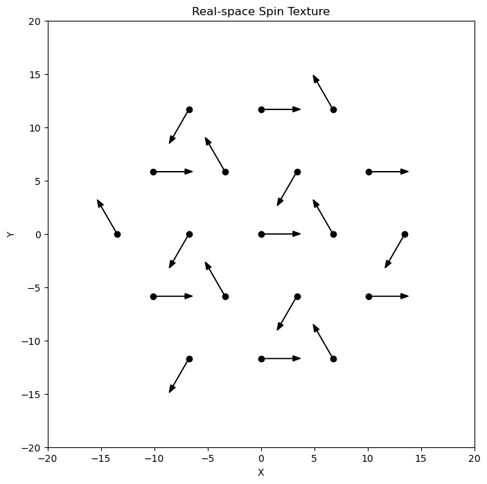
plt.show()

The above will give a figure like follows, which confirms the stripe phase corresponding to the \mathbf{q} vector being the M point:

We also see the 120^\circ order for \mathbf{q} being the K point:

It goes without saying that you can use the above code to visualize the spin texture for any \mathbf{q} point (not necessarily the spin-spiral energy minimum).

We can use the previous tutorial I wrote, on getting an arbitrary number of lattice vectors, to visualize the spin texture for an even larger sample. For instance, for \mathbf{q}=(0.214286, 0.214286) (a random incommensurate vector):

The above was generated using the following code:

import pandas as pd
import numpy as np
import matplotlib.pyplot as plt

# Load the Excel file
file_path = "coords.xlsx" # Change this to match your file name
sheet_name = "coords" # Change this to match your sheet name (if .xlsx)
data = pd.read_excel(file_path, sheet_name=sheet_name)

# Extract coordinates
x = data['x25x25'].values # x25x25  
y = data['y25x25'].values # y25x25 

# Get the first atom's coordinates
x1, y1 = x[0], y[0]

# Calculate distances between the first atom and all other atoms
distances = np.sqrt((x - x1)**2 + (y - y1)**2)

# Round distances to 3 decimal places
distances_rounded = np.round(distances, 3)

# Get unique distances
unique_distances = np.unique(distances_rounded)

# Define lattice constant a
a = 6.744

# Divide all unique distances by a
scaled_distances = unique_distances / a 
squared_distances = np.round(scaled_distances**2, 2) # Square each scaled value

# Lattice Vectors
a1 = a * np.array([1, 0])
a2 = a * np.array([-0.5, np.sqrt(3) / 2])

# Reciprocal lattice vectors (hardcoded)
b1 = np.array([6.283185307179587, 3.627598728468436]) / a
b2 = np.array([0., 7.255197456936872]) / a

# Fixed q-point
q = np.array([0.214286, 0.214286])  
q_physical = q[0] * b1 + q[1] * b2

# Parameters
mx, my, mz = 1, 0, 0 # Initial mx,my,mz
# Define S[q, R]
def S(q, R):
    q_dot_R = np.dot(q, R)
    return np.array([
        mx * np.cos(q_dot_R) - my * np.sin(q_dot_R),
        mx * np.sin(q_dot_R) + my * np.cos(q_dot_R)
    ])
# Function to compute R vectors based on target squared magnitude
def get_R(target_squared_magnitude):
    R_cartesian = []
    for n1 in range(-50, 50):  # Expand search range if needed
        for n2 in range(-50, 50):
            squared_magnitude = n1**2 + n2**2 - n1 * n2
            if np.isclose(squared_magnitude, target_squared_magnitude, atol=1e-7):  # Allow small tolerance
                R = n1 * a1 + n2 * a2
                R_cartesian.append(R)
    return np.array(R_cartesian)
# Plotting function
plt.figure(figsize=(10, 10))
# Loop over each squared distance and add to the plot
for g in squared_distances:
    R = get_R(g)  # Get R vectors for the current squared distance
    if R.size == 0:
        print(f"No R vectors found for squared distance: {g}")
        continue
    S_vectors = np.array([S(q_physical, r) for r in R])
    # Plot the arrows
    plt.scatter(R[:, 0], R[:, 1], color='black', s=10)
    scale_factor = 3
    for i in range(len(R)):
        normalized_S = scale_factor * S_vectors[i] / np.linalg.norm(S_vectors[i]) if np.linalg.norm(S_vectors[i]) != 0 else S_vectors[i]
        plt.arrow(
            R[i, 0], R[i, 1], normalized_S[0], normalized_S[1],
            color='black', head_width=0.5, head_length=0.7
        )
        
R_origin = np.array([0, 0]) # Define the R vector for the origin
S_origin = S(q_physical, R_origin)
scale_factor = 3  # Same scale factor as used for other arrows
normalized_S_origin = scale_factor * S_origin / np.linalg.norm(S_origin) if np.linalg.norm(S_origin) != 0 else S_origin
plt.scatter(R_origin[0], R_origin[1], color='black', s=10)
plt.arrow(
    R_origin[0], R_origin[1], normalized_S_origin[0], normalized_S_origin[1],
    color='black', head_width=0.5, head_length=0.7, label='Arrow at Origin'
)
plt.gca().set_aspect('equal', adjustable='box')
plt.xlim(-175, 175) 
plt.ylim(-175, 175)
plt.xlabel("X")
plt.ylabel("Y")
plt.title("Real-space Spin Texture")
#plt.legend()
plt.grid(False)
plt.show()

Hope you find this useful!